stravadata is an R package I use to organize and analyze my Strava activity data. This post offers some example analyses:
- Computing annual totals
- Making activity heat maps
- Counting efforts
- Making training calendars
- Tracking personal records
My examples use data on my running activities from the last five years:
library(dplyr)
library(lubridate)
library(stravadata)

runs = activities %>%
  filter(type == 'Run') %>%
  mutate(year = year(start_time),
         date = date(start_time)) %>%
  filter(year %in% 2018:2022)
Computing annual totals
runs contains activity-level features like distance traveled and time spent moving.
I sum these features by year, then use knitr::kable to display these sums in a table:
library(knitr)

runs %>%
  group_by(Year = year) %>%
  summarise(Runs = n(),
            `Distance (km)` = sum(distance) / 1e3,
            `Time (hours)` = sum(time_moving) / 3600) %>%
  mutate_at(3:4, ~format(round(.), big.mark = ',')) %>%
  kable(align = 'crrr')
| Year | Runs | Distance (km) | Time (hours) |
|---|---|---|---|
| 2018 | 68 | 544 | 52 |
| 2019 | 152 | 1,085 | 92 |
| 2020 | 224 | 2,026 | 172 |
| 2021 | 207 | 2,149 | 173 |
| 2022 | 145 | 1,517 | 120 |
Making activity heat maps
I record my runs with a watch that tracks my GPS coordinates.
stravadata stores these coordinates in streams.
For example, here’s the course for last year’s Moonlight Run in Palo Alto:
library(ggplot2)

p = runs %>%
  filter(name == 'Moonlight Run' & year == 2022) %>%
  select(id) %>%
  left_join(streams, by = 'id') %>%
  ggplot(aes(lon, lat)) +
  geom_path()

plot_nicely(p)  # Add text and formatting

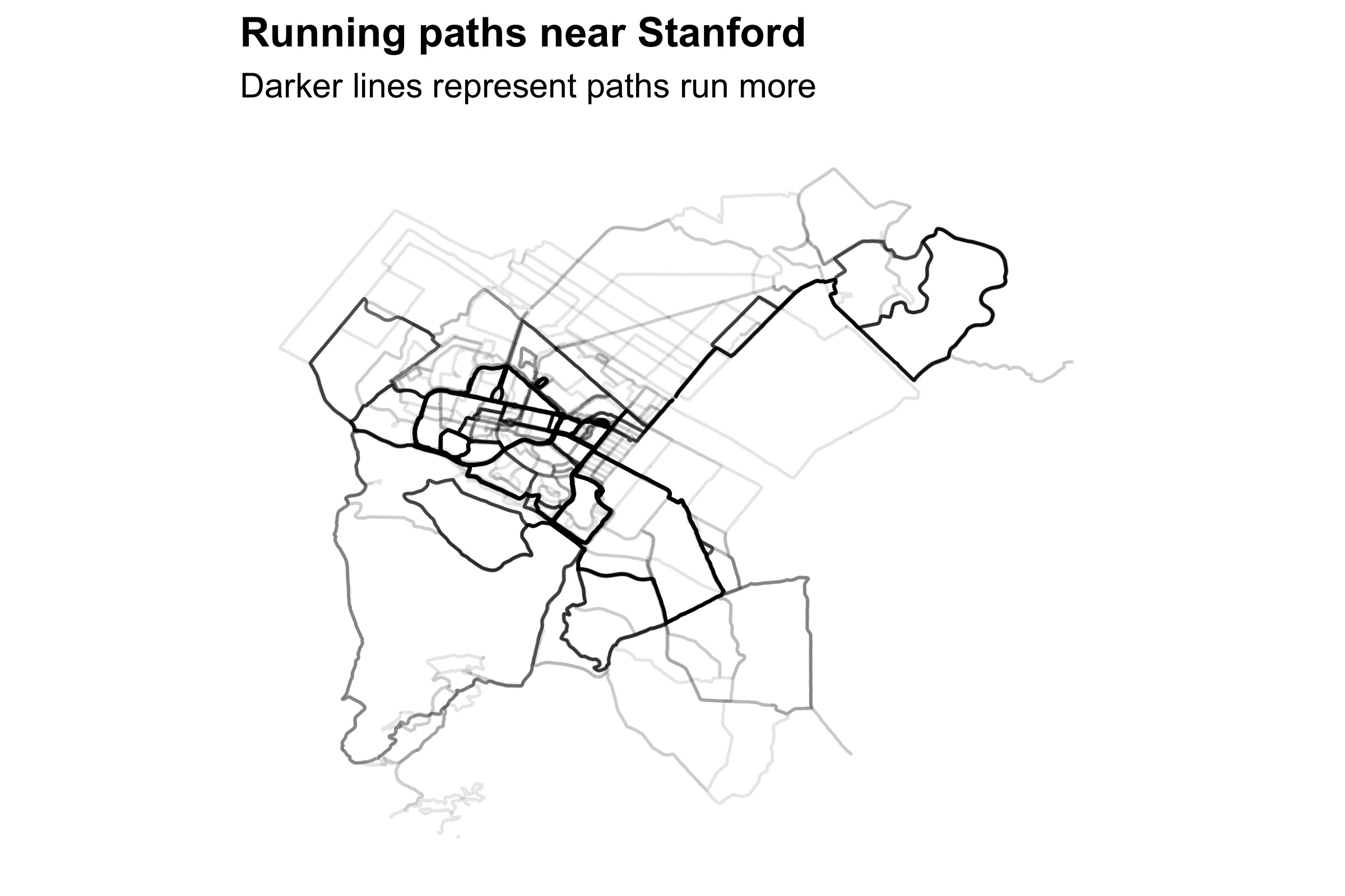
Combining the GPS coordinates from many runs yields a local map. For example, suppose I want to map my runs near Stanford. I first make a table of GPS paths near a local landmark:
coords = c(-122.16, 37.44)  # Trader Joe's
tol = 0.08

stanford_paths = streams %>%
  semi_join(runs, by = 'id') %>%
  mutate(step = row_number()) %>%
  filter(sqrt((lon - coords[1]) ^ 2 + (lat - coords[2]) ^ 2) < tol) %>%
  filter(lon != lag(lon) | lat != lag(lat)) %>%  # Remove pauses
  mutate(new_path = row_number() == 1 | id != lag(id) | step != lag(step) + 1) %>%
  mutate(path = cumsum(new_path)) %>%
  select(path, lat, lon)
I increment path every time I start a new run, unpause a previous run, or re-enter the area defined by coords and tol.
I use path as a grouping variable so that ggplot2::ggplot knows to draw each path separately.
I then use the alpha argument of ggplot2::geom_path to create a “heat map” of paths I run most often:
p = stanford_paths %>%
  ggplot(aes(lon, lat, group = path)) +
  geom_path(alpha = 0.1)

plot_nicely(p)
Counting efforts
best_efforts stores my fastest times running a range of distances (that Strava calls “efforts”) within each activity:
head(best_efforts)
## # A tibble: 6 × 4
##           id effort   start_index end_index
##        <dbl> <chr>          <int>     <int>
## 1 1253004287 1 mile            15       447
## 2 1253004287 1/2 mile          11       232
## 3 1253004287 1k                12       284
## 4 1253004287 2 mile            11       876
## 5 1253004287 400m              11       120
## 6 1253004287 5k                11      1342
The id column stores activity IDs and the effort column stores effort descriptions.
I focus on 5k, 10k, and half marathon efforts:
focal_efforts = c('5k', '10k', 'Half-Marathon')

efforts = runs %>%
  left_join(best_efforts, by = 'id') %>%
  filter(effort %in% focal_efforts) %>%
  mutate(effort = factor(effort, focal_efforts)) %>%
  select(year, date, id, effort, start_index, end_index)
efforts inherits the year variable from runs.
I use this variable to count efforts within each year.
I then use tidyr::spread and knitr::kable to display these counts in a table:
library(tidyr)

efforts %>%
  count(Year = year, effort) %>%
  spread(effort, n, fill = 0) %>%
  kable(align = 'c')
| Year | 5k | 10k | Half-Marathon |
|---|---|---|---|
| 2018 | 64 | 24 | 0 |
| 2019 | 136 | 34 | 2 |
| 2020 | 191 | 88 | 21 |
| 2021 | 200 | 90 | 25 |
| 2022 | 131 | 85 | 9 |
Making training calendars
efforts also inherits the date variable from runs.
I use this variable to create GitHub-esque training calendars.
For example, here’s my running calendar for 2021:
p = efforts %>%
  filter(year == 2021) %>%
  group_by(date) %>%
  slice_max(effort) %>%
  distinct(effort) %>%  # I ran twice on some days
  mutate(Week = floor_date(date, 'weeks', week_start = 1),
         Weekday = wday(date, label = T, week_start = 1)) %>%
  ggplot(aes(Week, Weekday)) +
  geom_tile(aes(alpha = effort), col = 'white', linewidth = 0.5)

plot_nicely(p)

I use lubridate::floor_date to identify weeks and lubridate::wday to identify weekdays.
The col and size arguments of ggplot2::geom_tile add space between tiles.
Tracking personal records
I combine runs, streams, and efforts to track my record running paces over time.
I follow a three-step process:
First, I compute the mean pace for each effort.
I do this using the start_index and end_index columns that efforts inherits from best_efforts.
These columns tell me where each effort occurs in the corresponding activity’s stream:
effort_paces = streams %>%
  filter(id %in% runs$id) %>%
  # Create indices
  group_by(id) %>%
  mutate(index = row_number()) %>%
  ungroup() %>%
  # Extract stream segment for each effort
  inner_join(efforts, by = 'id') %>%
  filter(index >= start_index & index <= end_index) %>%
  # Compute mean paces
  group_by(id, date, effort) %>%
  summarise(distance = max(distance) - min(distance),
            time = max(time) - min(time)) %>%
  ungroup() %>%
  mutate(pace = (time / 60) / (distance / 1e3))

head(effort_paces)
## # A tibble: 6 × 6
##           id date       effort distance  time  pace
##        <dbl> <date>     <fct>     <dbl> <dbl> <dbl>
## 1 1335437333 2018-01-01 5k        5002.  1442  4.81
## 2 1338123783 2018-01-03 5k        5000.  1605  5.35
## 3 1344338907 2018-01-07 5k        5000.  1455  4.85
## 4 1347622521 2018-01-09 5k        5000   1493  4.98
## 5 1353889714 2018-01-13 5k        5001.  1622  5.41
## 6 1353889714 2018-01-13 10k      10001.  3380  5.63
The values in the distance column differ slightly from the descriptions in the effort column.
This is because the stream segment doesn’t always cover the described distance exactly.
But the multiplicative errors in distance and time should be equal on average, making pace is an unbiased estimate of my true mean pace.
I measure this pace in minutes per kilometer.
Next, I extract my record paces by deleting efforts slower than my previous best:
record_paces = effort_paces %>%
  group_by(effort) %>%
  arrange(date) %>%
  filter(pace == cummin(pace)) %>%
  ungroup()
Finally, I “fill in the gaps” by adding days on which I don’t set a new record.
I do this using tidyr::crossing and tidyr::fill:
date_range = seq(date('2018-01-01'), date('2022-12-31'), by = 'day')

record_paces_filled = crossing(date = date_range, effort = focal_efforts) %>%
  left_join(record_paces) %>%
  group_by(effort) %>%
  fill(pace) %>%
  filter(!is.na(pace))
record_paces and record_paces_filled differ in that the latter includes date-effort pairs with no new records.
This makes record_paces_filled produce horizontal lines when I plot its data:
p = record_paces_filled %>%
  ggplot(aes(date, pace, group = effort)) +
  geom_line()

plot_nicely(p)
